In a previous post I showed a simple way to control for language family and area with categorical variables in a linear mixed model using Python. In a more recent post I showed how we can plot languages on a map based on various features such as word order and language family. The use of “macroareas” as a control for potential language contact is not ideal, as it treats all languages within a given area as having the same relationship. However, “macroareas” are a better option than no areal control at all, and while I will consider other options in a future post, this post focuses on how such areas are derived.

The Glottolog database has identified macroareas for languages of the world. These six areas include Eurasia, Africa, Papunesia, North America, South America, and Australia, and are justified by Hammarström & Donohue (2014) as meeting necessary criteria for geographical independence. Another way of deriving areas is by clustering - using an algorithm such as K-means to determine the number of groups that best accounts for variance in a set of GPS coordinates. The remainder of this post illustrates and compares the two approaches using maps, with some discussion about the benefits of each.

Getting the data

As with previous tutorials, I’m assuming that you’ve set up a Python 3.10 environment and have some familiarity with writing and running Python scripts (i.e. via a terminal). For a basic setup tutorial, you can follow these instructions.

For our purposes, we first want to observe how the six macroareas look when we map them based on GPS coordinates. Glottolog has information for languages grouped into macroareas along with latitude and longitude. The following python code downloads the data from Glottolog and stores it in a file in your local directory, then loads it using pandas so that we can visualize the data structure in the terminal.

import os, requests # for file handling
import pandas as pd # for data processing

glottofile = "Glottolog_Languages.csv" # comma-separated file with glottocodes and other info
# check whether the file exists already
if not os.path.isfile(glottofile):
    # use the raw bitstream URL for this file
    url = "https://cdstar.eva.mpg.de//bitstreams/EAEA0-608B-9919-A962-0/languages_and_dialects_geo.csv"
    # fetch the file content
    response = requests.get(url)
    # write content to the local file
    if response.status_code == 200:
        with open(glottofile, "wb") as file:
            file.write(response.content)
        print("Download complete!")
    else:
        print(f"Failed to download. Status code: {response.status_code}")
else:
    print("File exists!")

gldf = pd.read_csv(glottofile) # read in the dataset
print(gldf.head()) # check its structure
print(f'There are {len(gldf)} languoids in the dataset')
print(gldf.macroarea.value_counts()) # print the macroareas and how many languoids in each area

# File exists!
#
#   glottocode        name isocodes     level  macroarea  latitude  longitude
# 0   3adt1234  3Ad-Tekles      NaN   dialect     Africa       NaN        NaN
# 1   aala1237      Aalawa      NaN   dialect  Papunesia       NaN        NaN
# 2   aant1238  Aantantara      NaN   dialect  Papunesia       NaN        NaN
# 3   aari1239        Aari      aiw  language     Africa   5.95034    36.5721
# 4   aari1240      Aariya      aay  language    Eurasia       NaN        NaN
#
# There are 22324 languoids in the dataset
#
# macroarea
# Eurasia          7116
# Africa           6581
# Papunesia        5149
# North America    1453
# South America    1229
# Australia         704
#

Plotting languages by Glottolog macroarea

Here we can see that there are over 22k data points in the dataset, but not all of them correspond to individual languages (some are classed as dialects, for example), and not all of them have GPS coordinates (latitude and longitude). We can also see that some macroareas are much better represented than others. In the following code we can reduce the dataset to only those language varieties with GPS coordinates.

gldf = gldf.dropna(subset=['latitude']) # drop data that doesn't contain latitude info
print(f'There are {len(gldf)} languoids in the dataset with latitude info')
print(gldf.macroarea.value_counts()) # print the macroareas and how many languoids in each area

# There are 8889 languoids in the dataset with latitude info
#
# macroarea
# Africa           2418
# Papunesia        2281
# Eurasia          2251
# North America     795
# South America     703
# Australia         441
#

This leaves us with nearly 9k data points, and the following code plots them on an interactive map. In this blog post I reproduce only the image, but running this code locally will display an html page that allows you to click and zoom.

import plotly.express as px # the plotting package
import colorcet as cc # the color package

# create the scatter map
fig = px.scatter_geo(
    gldf,                             # the dataframe containing our data
    lat="latitude",                   # name of the column with latitude values
    lon="longitude",                  # name of the column with longitude values
    color="macroarea",                # macroarea column dictates color
    hover_name="name",                # name of the language for visualization
    projection="natural earth",       # map projection used by plotly
    title="Languages by Macroarea",   # title of the map
    color_discrete_sequence=cc.glasbey_dark, # set of distinctive colors (from 256)
)

# display the map in a browser
fig.show()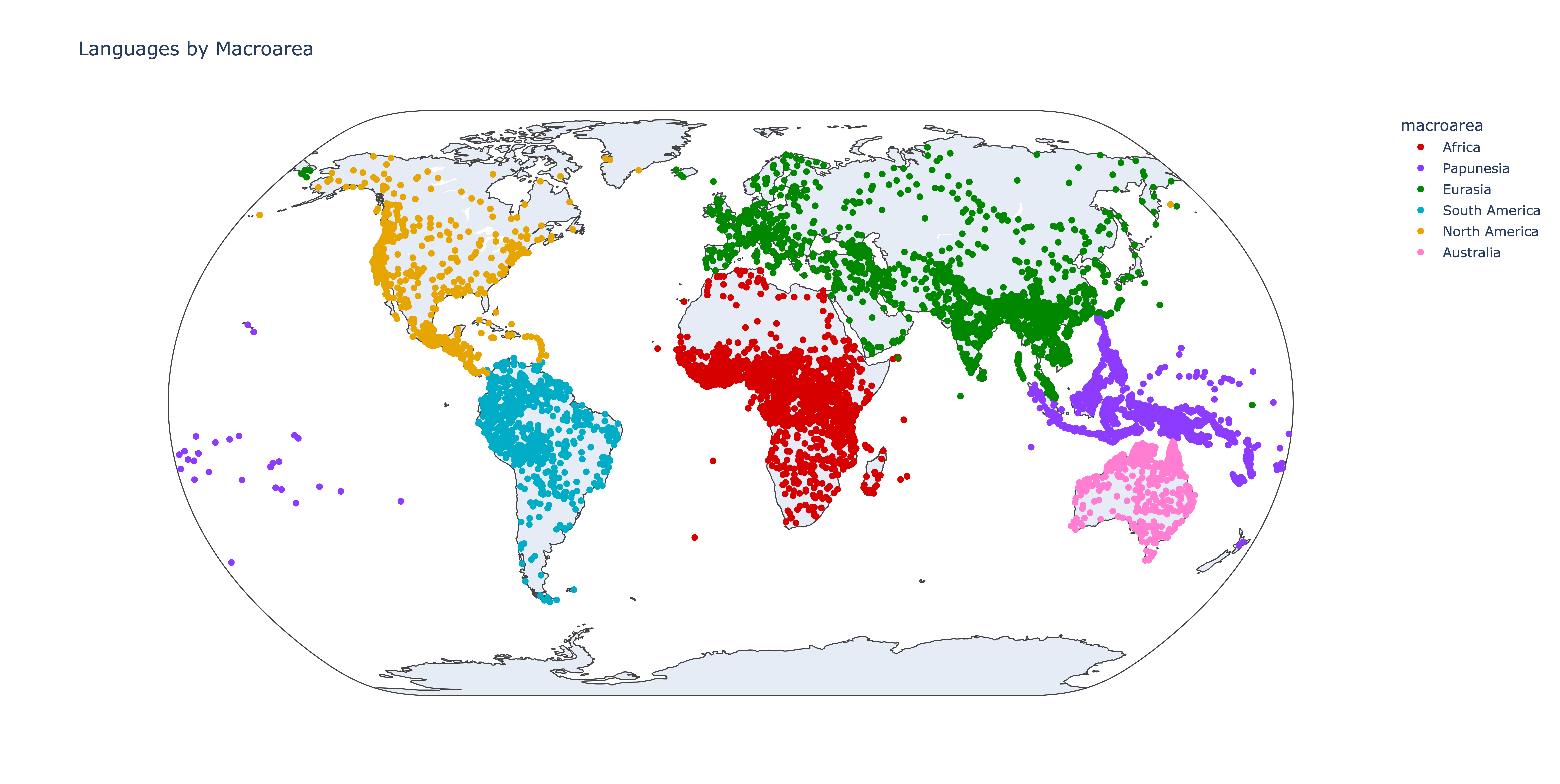

From the map, we can see that these macroareas line up very well with the major landmasses, with only a few possible exceptions (like Chinese Pidgin English which is classed as belonging to the “Eurasian” macroarea despite sharing a location with Nauru in the Pacific).

As noted in the 2014 paper, this set of macroareas is intended to provide a foundation, based on our knowledge of possible interactions between humans. The essential observation is that areas which share landmass are more likely to see contact between groups and therefore between speakers of different languages. The exception to such a rule is when technology (such as sailing vessels for the Austronesians) enables contact across vast distances (i.e. oceans) or difficult-to-cross barriers (i.e. mountains).

Deriving and plotting macroareas by geographic coordinates

Another way to derive areas is by clustering data according to distance between coordinates. There are two general ways to do this, both of which require transformation of the coordinates to feed to a clustering algorithm. The first method involves conversion to Hilbert distances, and the second to Cartesian space. While both can be done relatively easily using Python, Hilbert distances (due to their 1D nature) can suffer from “boundary discontinuities” and lead to problems with clustering algorithms, whereas Cartesian coordinates lend themselves better to clustering methods.

The following code first converts latitude and longitude of all the languoids in the dataset to 3D Cartesian space, and then fits a series of K-means clusters, using the silhouette score to identify the optimal number of clusters.

import numpy as np
from sklearn.cluster import KMeans
from sklearn.metrics import silhouette_score
from sklearn.preprocessing import StandardScaler

def get_clusters(df):
    """A function to determine optimal number of clusters from lat, long"""
    # conversion to 3D Cartesian space
    lat_rad = np.radians(df['latitude'])
    lon_rad = np.radians(df['longitude'])

    df['X'] = np.cos(lat_rad) * np.cos(lon_rad)
    df['Y'] = np.cos(lat_rad) * np.sin(lon_rad)
    df['Z'] = np.sin(lat_rad)

    features = df[['X', 'Y', 'Z']].values

    # z-score standardization
    scaler = StandardScaler()
    scaled_features = scaler.fit_transform(features)

    # iterative silhouette evaluation
    silhouette_scores = {}
    k_range = range(2, 20)  # Checking 2 to 20 potential geographic language macro-areas

    for k in k_range:
        kmeans = KMeans(n_clusters=k, random_state=42, n_init=20)
        labels = kmeans.fit_predict(scaled_features)

        score = silhouette_score(scaled_features, labels)
        silhouette_scores[k] = score
        print(f"Macro-Clusters (K): {k} | silhouette coefficient: {score:.4f}")

    # extract optimal number of clusters
    optimal_k = max(silhouette_scores, key=silhouette_scores.get)
    print(f"Optimal geographic language clusters: K = {optimal_k}")

    print(f"Trying with K = {optimal_k}")

    # apply final model and put each language in its cluster
    final_model = KMeans(n_clusters=optimal_k, random_state=42, n_init=20)
    df['K_macroarea'] = final_model.fit_predict(scaled_features)

    return df

# run the function on the `gldf` dataframe
gldf = get_clusters(gldf)

You should see that the optimal number of clusters identified through this method is six, which is the same number of macroareas used in the Glottolog dataset. We can now proceed to plotting the languages based on the newly-identified clusters, with the following code.

clusters = "K_macroarea" # column for grouping
gldf[clusters] = gldf[clusters].astype(str) # convert to categorical (number to string)

# create the scatter map
fig = px.scatter_geo(
    gldf,                             # the dataframe containing our data
    lat="latitude",                   # name of the column with latitude values
    lon="longitude",                  # name of the column with longitude values
    color=clusters,                   # cluster column dictates color
    hover_name="name",                # name of the language for visualization
    projection="natural earth",       # map projection used by plotly
    title=f"Languages by {clusters}", # title of the map
    color_discrete_sequence=cc.glasbey_dark, # set of distinctive colors (from 256)
)

fig.show() # display the map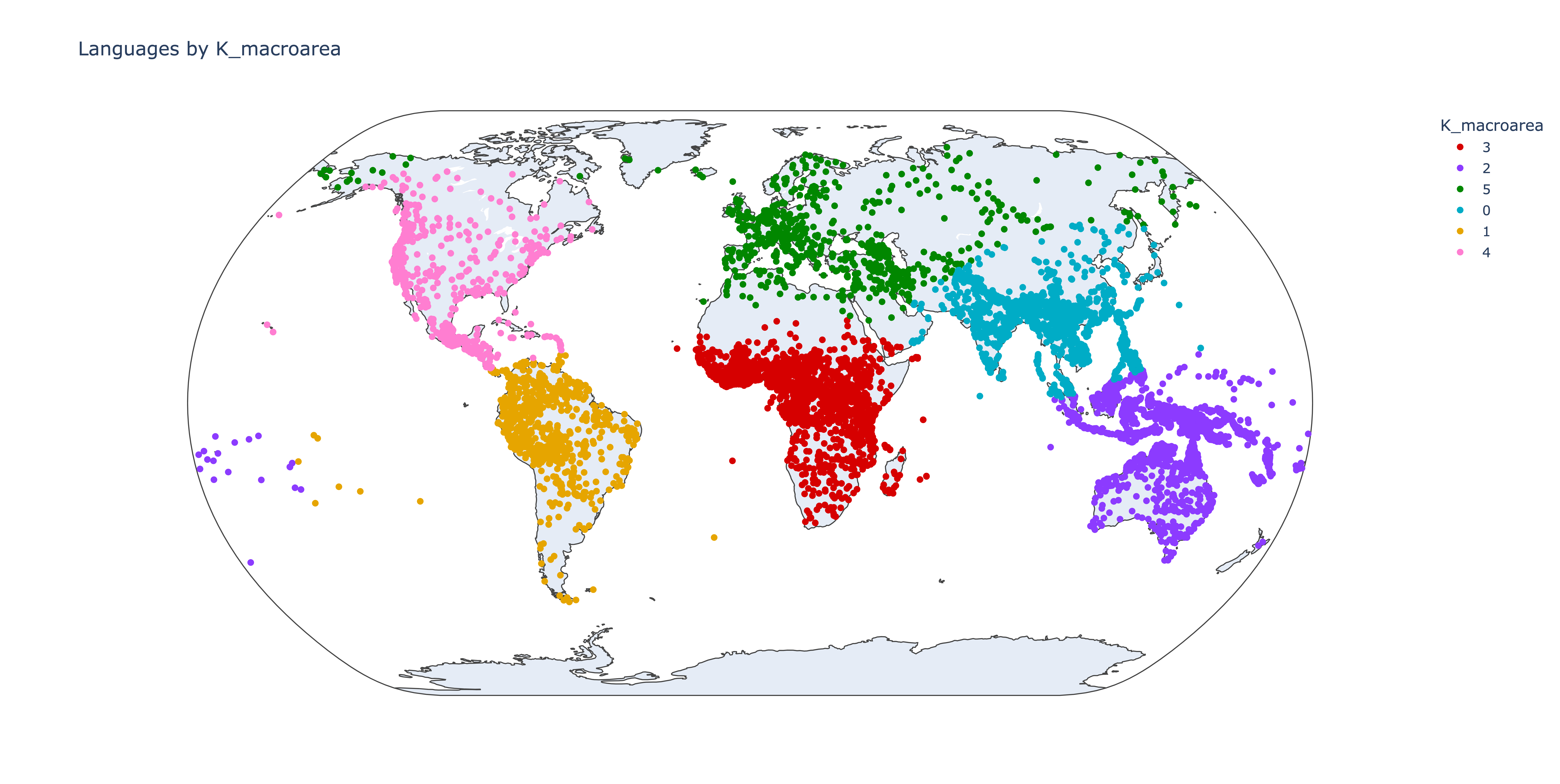

This gives us an interactive map, corresponding to the image above. Comparing this map with the Glottolog macroareas map, there are several observations. The first is that both identify 6 clusters, but in slightly different ways. Glottolog’s macroareas separate Australia from Papunesia/Oceania, while the K-means clustering combines these but separates Asia from Eurasia. A second observation is that some island oceanic languages are grouped with the Americas by the K-means clsuters, in opposition to the Glottolog macroareas. A third thing to notice is that some languages in the arctic are classified differently by the K-means meathod than by Glottolog. A final point is that a few individual languages seem to be oddly colored by the Glottolog grouping, such as Chinese Pidgin English identified above.

Discussion

The fact that the two ways of identifying geographical clusters for languages are so similar is quite striking. Intuitions and expert determinations of “language area” seem in this sense to align quite well with a more naive mathematical approach. You could make an argument that the K-means geographical groupings are actually better in some ways - aligning with real barriers to population movement, such as the Himalayan mountain range and the Wallace Line. Even the K-means grouping of some Oceanic languages with the Americas is plausible, given that contact is attested from at least the 1200s (see also DNA studies).

However, these groupings could also be somewhat spurious. History indicates that humans often find reasons to overcome apparent obstacles, such as when motivated by trade and resources. At the same time, there is much to be said for ease of movement, which geographical proximity facilitates. In the case of the Glottolog macroareas, there are reasonable theoretical reasons for creating these particular groupings, as highlighted in Hammarström & Donohue (2014).

One additional question is how well these slightly different geographical groupings facilitate downstream investigations. The Glottolog macroareas are regularly used in typological studies as categorical grouping variables to control for contact. The K-means Cartesian clusters have yet to be used for this, though I am working on a paper to compare the different groupings. Another common way of controlling for area is by using a Gaussian process term, though this is generally used along with a categorical grouping variable (i.e. macroareas), as I will discuss in a future post. One benefit of the unsupervised clustering approach is that it could potentially be applied to any geographical area, given enough data points, as I discuss in a current working paper.

In the end, it may be best to combine insights derived both from theoretical positions (and our knowledge of human history and migration) as well as from mathematical approaches such as K-means clustering. Each perspective can inform the other, and as we develop better ways of organizing and analyzing our data, this will help us get closer to understanding how languages change.